Event-based computing with
dendritic plateau potentials

Neurons can do much more than we give them credit for. Or rather: much more than current neural network models give them credit for. In this blog post, I want to motivate and explain a simple neuron model that Pascal Nieters, Gordon Pipa and I developed ｢1｣ to make sense of temporal dynamics in active dendrites and their role for computation.

This page contains interactive elements that may take a while to load properly!

Since neurons were first discovered more than a century ago, we have learned a lot about their structure, connectivity and internal processes. But these insights have had surprisingly little impact on the development of artificial neural network models, which have taken the world by storm in recent years. Even in the area of the spiking neural networks, which are more popular in theoretical neuroscience than they are in artificial intelligence, we commonly work with neuron models that have changed little over the last 50 years.

The most influential and widely used spiking neuron models to date are the leaky-integrate-and-fire (LIF) model and its variants. This is not surprising considering its simplicity, nice mathematical properties and the fact that it can be derived from a few biological first principles. But the last two decades of neuroscience have uncovered phenomena that the LIF neuron cannot account for, including the fascinating role that active processes in dendrites play for integrating information and learning.

In a recent publication｢1｣, Pascal Nieters, Gordon Pipa and I set out to make sense of these findings. This lead us to a very simple yet powerful neuron model that I want to present in the following. But before we get there, I’d like to briefly recap the motivation behind the LIF neuron model and then try to poke some holes into it.

From first principles to LIF neurons

Each neuron is filled with and surrounded by liquid, and in this liquid, there are various ions (e.g. sodium, Na⁺, potassium, K⁺, chloride, Ch⁻, and calcium, Ca²⁺) at various concentrations. These ions move around stochastically due to thermal energy, and they attract or repel each other, depending on their electric charge. If it weren’t for the neuron’s cell membrane, the ions would diffuse over time, and their concentrations inside and outside the cell would equilibrate. But the membrane is a very effective barrier for these ions, and specific ion pumps inside the neuron’s membrane work tirelessly to maintain or restore an imbalanced distribution of ions. A neuron at rest is thus “pumped up” and ready to respond quickly to any input.

When a synaptic spike arrives, it triggers the release of neurotransmitters that briefly open channels in the neuron’s membrane, which can let specific ions pass. Due to the great differential in concentration and electric potential, the ions now rush out of (or into) the cell, like air leaving an inflated balloon; but unlike a balloon, the channel can be selective for a specific type of ions. For example, if a channel only lets sodium ions pass, they will rush into the cell, where the concentration is much lower, and thus increase the electric potential inside the cell. If a channel mainly lets potassium ions pass, they will rush out of the cell and thus reduce the potential. Letting the ions of specific type flow freely brings the neuron towards a new equilibrium, where the pull exerted on the ions by the electric field across the membrane exactly compensates for the stochastic diffusion of ions through the channel along the chemical concentration gradient.

If we now think of the neuron’s membrane as a capacitor, each spike thus adds or subtracts a charge, depending on which channels are opened. This can be approximated by assigning to each synapse a weight or efficacy that determines how much (ionic) current a spike will inject into the neuron¹. In this simplified world, the effect is completely linear: the larger a synapse is, the more channels it will open, and the stronger the effect will be. Likewise, the effect of multiple synapses sums up, and charges are accumulated (integrated) over time. But since the membrane is not a perfect insulator and the channels don’t close perfectly (and also considering the effect of ion pumps), these charges will leak out slowly over time.

If the membrane potential at some point crosses a critical threshold voltage, other voltage-gated ion channels start opening (e.g. for sodium ions). This increases the membrane potential further, leading to a positive feedback-loop that quickly discharges or depolarizes the neuron. When this happens, the neuron will first fire out a spike (a self-propagating electric wave) along its axon; then the net-flow of charges through the open channels reverses, as a different type of ion flow starts to dominate (e.g. potassium ions). This resets the neuron’s membrane potential back down to its initial level. The tireless ion pumps then re-establish the original ion distribution, using energy to pump Na⁺ out of and K⁺ into the cell and thus make the neuron ready for its next spike. Hence the name of the model, leaky integrate-and-fire neuron.

In simpler words, this model is just a linear first-order filter followed by a non-linear threshold detection. For any electrical engineers, this might be familiar from signal processing as $\Sigma\Delta$‑modulation. Now throughout this entire section, I have treated the neuron as a little “ball” with a homogeneous in- and outside, and a membrane separating the two. This class of models² is, therefore, called point-neurons to emphasize the fact that they only model the neuron at a single point in space, typically assumed to be at the soma. Of course, we know that real neurons have quite elaborate spatial structures, so we will later question if this simplification is really justified. But locally, the mechanism described above is a good first approximation of how a neural membrane behaves.

Neurons as coincidence detectors

Now what computation does such a neuron perform, intuitively? Well, to be as general as possible, we could say that the neuron’s state, i.e. its membrane potential $V(t)$, holds some information about the history of inputs that the neuron has seen. We could formalize this rigorously in the language of probability theory.³ But such a definition is awfully complex, and does not really explain how another neuron would make use of this information.

Luckily, we can find a much simpler interpretation if we assume that the accumulated charges leak out of the neuron within a few milliseconds, and that neurons only fire a handful of spikes per second (which is true for most neurons). Then, the effect of one synapse’s previous spike vanishes before its next spike arrives, and we don’t need to consider the effect of more than one spike per synapse. That means, that the neuron’s membrane potential can only make it above the threshold if sufficiently many spikes arrive through sufficiently strong synapses in a sufficiently brief time-window. In other words: the LIF neuron is a simple coincidence detector that fires whenever it receives a lot of input in a short amount of time!

Now, on first glance, coincidence detection is a plausible function of a neuron; after all, we need to be able to relate various sensory inputs to each other. But I would argue that this form of coincidence detection is too simple to be useful. To show that, let’s consider a few examples.

Integrating information from different modalities

As we saw above, a single LIF neuron can detect coincident spikes on the timescale determined by its leak-rate, which depends on physical properties of the neuron such as the conductance and capacitance of the membrane. For example, if it takes the neuron’s membrane potential around $10\text{ms}$ to decay from close-to-threshold to below the noise floor, then the neuron can easily detect two coincident spikes from synapses $a$ and $b$ if they arrive within around $5\text{ms}$ of each other. To do this, the two synaptic weights must be high enough that two near-simultaneous spikes push the membrane potential above the threshold, but not so high that either spike alone is sufficient. This type of tight coincidence detection makes sense if the two synapses carry signals that are precisely aligned in time, e.g. if they come two neighboring rods in the retina, or two neighboring hair cells in the ear.

But what if the two synapses come from two different neuron populations or sensory modalities, e.g. one comes from visual, the other from auditory cortex? It seems unlikely that these two spikes would be aligned on such a precise timescale. Instead we might want to detect “coincident” spikes that are much more - say, $50 \text{ms}$ - apart. The LIF neuron above forgets too quickly to cover such a long time interval. Now we could try to salvage that by increasing the neuron’s time constant, but even if we slowed it down by a lot, the same mechanism wouldn’t work: if we slowed the membrane time-constant to $50 \text{ms}$ or more, it could reliably detect two far-apart spikes, but then either synapse $a$ or $b$ could in fact fire multiple spikes in that time interval, and the neuron has no way of distinguishing between them. The neuron could thus not distinguish between co-activation of two different modalities, or excessive activation of just one of them.

Detecting the order of spikes

Now assume that we are not only interested in the coincidence of spikes, but also in their temporal order. For example, activating two neighboring rods on the retina in a specific order might indicate movement in one direction, while activating the same rods in reverse order might indicate movement in the opposite direction.

Point neurons can detect such subtle timing-differences if we allow for different transmission delays. For example, if synapse $a$ is delayed by $5 \text{ms}$ relative to $b$, then our coincidence detecting neuron will fire whenever $a$’s neuron fires around $5 \text{ms}$ before $b$’s neuron.

But this implies that the exact delay between the two is a) known in advance and b) somehow hard-coded into the transmission delay. If we want to detect the order of spikes with invariance to their precise timing, we need a different mechanism. Besides, transmission delays in cortex are only on the order of a few milliseconds, which means that this mechanism cannot explain the detection of temporal orders of spikes on the much slower timescales needed for multi-modal integration.

Crossing multiple time-scales

Finally, let’s consider what happens if we want to cross multiple time-scales. For example, assume that we’d like to detect two events, first $A$ and then $B$, where each of these two events is encoded by a volley of coincident spikes from neuron population $(a_1,a_2)$ and $(b_1,b_2)$, respectively. One coincidence detecting neuron each could perform the detection of the two events. To detect that $A$ occurred before $B$, we’d then need a third neuron with a much slower inherent timescale to integrate the information from the first two.

This implies that networks of spiking neurons and synapses should have a diverse set of inherent timescales, but these parameters are static properties of the neuron. If we want to be able to detect the temporal order of events independently of the precise delays, we’d need a lot of carefully tuned neurons.

Hodgkin-Huxley to the rescue?

These examples are meant to highlight some limitations of point-neuron models, which motivated us to look for something better. Of course, there are already much more refined neuron models, e.g. detailed multi-compartment models based on the more involved Hodgkin-Huxley equations, including nonlinear effects and measurements of parameters like ion-channel densities from real neurons. But these bio-physically accurate models can have so many parameters that parameterizing them becomes an art in and of itself; and given the complexity of the model, merely reproducing an effect in simulation does not help much for understanding it.

Instead, we tried the proverbial wisdom to “make it as simple as possible, but no simpler”.⁴. Going back to first principles, we derived a different, yet conceptually simple account of how a spiking neuron might work. I’ll give an abridged version of these arguments in the next section.

Warning: To keep the biological background to a minimum, I cut a few corners here. You can find a more thorough explanation with references in ｢1｣.

The biological evidence

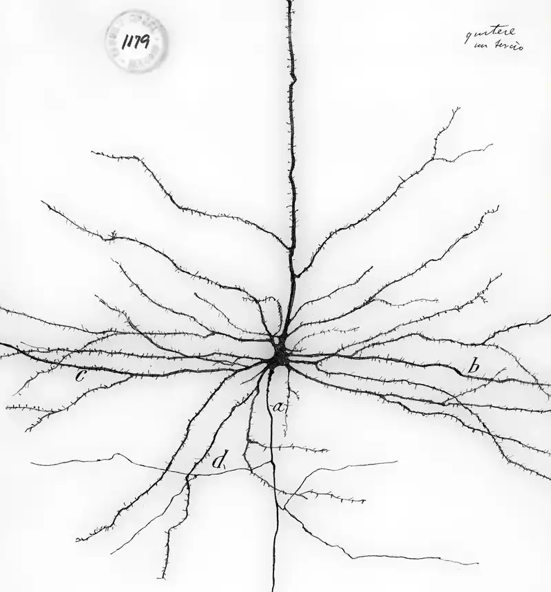
When we look back at Cajal’s drawing above, the stunningly complex dendrites immediately stand out. They comprise many branches of different length and thickness, and on each of these branches we can see countless dendritic spines. On these spines, synaptic connections to other neurons are formed⁵.

If we could look at one of these spines through an electron microscope, we would see that it packs a combination of different types of ion channels, most notably among them channels that are gated by AMPA and NMDA receptors. This, too, appears to serve some purpose, as there are lots of different channel and receptor types for the neuron to choose from, and yet we consistently find both of these on (distal) dendritic spines. Both channel types listen to the same neurotransmitter, Glutamate, and both let sodium and potassium ions pass, but only the NMDA channel also let’s calcium ions through. To complicate things further, the NMDA channels only open properly if the voltage is already elevated when the Glutamate arrives. In addition to these two types of channels, there are also voltage-gated calcium channels that seem to exacerbate the calcium influx once the membrane potential crosses some critical threshold.

The immediate effect of a synaptic spike on the targeted dendritic spine thus seems to be two-fold: on the one hand, we can observe an electric charge accumulating in the spine, caused by the in- and outward flow of sodium, potassium and calcium ions; on the other hand, the influx of calcium ions in particular appears to trigger a cascade of secondary messengers that can have some longer lasting effects.⁶

While the varying concentration of ions can be confined to the spine itself, the resulting electric field also affects the membrane potential of the dendrite branch itself. Sometimes, if a dendrite branch is excited a lot, e.g. by many simultaneous spikes or artificially by local glutamate uncaging, it seems to suddenly “switch on”, i.e. become depolarized. This phenomenon, called a plateau potential, can last for hundred(s) of milliseconds, and it seems to rely on NMDA channels and calcium influx. This is the fundamental mechanism on which we will build our neuron model. A plateau potential alone, however, is not enough to make a neuron fire; additional input further downstream is required.

If we now took two electrodes and used one to artificially change the voltage of some part of the dendrite, and used the other to record the effect of that intervention somewhere else, we’d notice a strong attenuation as we move the recording electrode closer to the soma. As we go in the opposite direction, the attenuation is much weaker. This is a consequence of the fact that the dendrite branches are tapered, such that the impedance along each branch slowly increases as we move away from the soma. A particularly strong impedance mismatch can be observed at branching points, which can even lead to a complete reflection of back-propagating action potentials.

So to summarize these observations, all of which have been known for decades:

• A cortical pyramidal neuron gets its input in the form of synaptic spikes.
• Synapses and dendritic spines seem to have evolved such that a pre-synaptic spike causes
  • an increase in the membrane potential of the dendritic spine
  • and a change in its calcium concentration.
• Membrane potentials spread passively but strongly attenuate on the way towards the soma.
• NMDA channels can have a strong depolarizing effect with considerable influx of calcium.
• Strong excitation can trigger long-lasting localized plateau potentials in dendrite branches.
• Elevated calcium ion concentration can have profound long-term effects, e.g. in learning.

What does this imply for neural computation? In the next section, we’ll put these pieces together and construct a very simple yet powerful model of spiking neurons, based on the nonlinear interaction of dendritic plateau potentials inside a neuron’s dendrites.

Our proposal

To make sense of the observations above, we believe a spiking neuron model should account for dendritic plateau potentials and their interaction across the dendrites. The model should thus incorporate the topology of the arbor and make predictions about its functional significance. This should provide answers about how a neuron (or a network of neurons) might be able to process temporally ordered sequences of spikes on variable, long and behaviorally relevant timescales. Let’s approach this goal step-by-step, starting again with a simplified point-neuron model.

Somatic spike = coincidence detection

Since the spike generation mechanism at the axon hillock is well understood, there is not much to change about it. Just like in the point neuron above, we thus say that the neuron will fire a spike, if it receives sufficiently many synaptic inputs in a sufficiently short amount of time - the soma acts as a coincidence detector! The only notable difference in our model is that we binarize the state of synapses for the sake of simplicity, i.e. we assume that the effect of a synaptic spike on the post-synaptic spine is constant throughout its duration, and that this effect wears off before the next spike can arrive on the same synapse.

You can see this behavior in the simulation below. The point-neuron receives input via two synapses $a_1$ and $a_2$, and it fires when both spikes co-occur within $3\text{ms}$ of each other - one spike alone is insufficient. Feel free to play around with the settings!

Plateau potential = coincidence detection + memory

Let’s now consider the same example as above, but this time, the synaptic inputs $a_1$ and $a_2$ target an (apical) dendrite segment $A$. As mentioned above, strong excitation of such a dendrite segment should induce a plateau potential there. In our model, we represent this by a very similar mechanism to the spike generation we are already familiar with: if sufficiently many synaptic inputs arrive within a sufficiently brief time-window, the dendrite segment enters a plateau state (again modeled by a binary variable) for a fixed amount of time. The crucial difference between somatic spikes and dendritic plateau potentials is, that the former are very short (a few milliseconds), whereas the latter can last up to a few hundred milliseconds! We can thus interpret the plateau potential as a memory trace of an event, where the event is represented by the coincidence of synaptic inputs.

The plateau potential corresponds to a very strong depolarization of the dendritic segment’s membrane potential, but this effect, as biological evidence shows, remains localized. That is why just the plateau potential is not enough to make the neuron fire a somatic spike in the simulation above. But how, then, do plateau potentials affect the operation of a neuron? We model this by a very simplistic gating mechanism.

Plateau potentials gate downstream dendrite segments

We know that membrane potentials diffuse along the dendrite, and that this diffusion strongly attenuates as we move towards the soma. Therefore, the effect of a strong depolarization in one dendrite segment, e.g. caused by a plateau potential, will weakly depolarize a neighboring downstream segment.⁷

This weak depolarization of the “parent” segment would then propagate to the next segment, and further on from there. With each “hop”, this passive spread is attenuated further. For the sake of simplicity, we assume that this effect quickly becomes negligible, so we only consider the effect of one segment on its direct neighbor. This effect can be modeled as raising the membrane potential of that segment to a level, where a moderate amount of coincident synaptic input can trigger a plateau potential. Without such depolarizing input from upstream, we assume that synaptic input alone can only trigger plateaus in apical / distal dendrite segments.

The effect of a dendritic plateau potential in one segment is thus to enable the next downstream segment, i.e. it acts as a gating mechanism. As we can see in the example above, the neuron fires a spike whenever the inputs $b_1$ and $b_2$ to the soma arrive while the dendrite segment $A$ is in a plateau state - in other words: the soma has to be triggered after the dendrite segment. The dendrite segment, in turn, only triggers a plateau when $a_1$ and $a_2$ spike simultaneously. This is extremely useful, because it allows us to detect not only coincident spikes, but also - you guessed it - ordered sequences of spikes!

Single neurons can detect long sequences of spikes

Now let’s consider a neuron with multiple dendrite segments that form a longer chain. Since each segment gates the next, such a neuron would only fire if all of its segments are activated in the correct order (and within the timing constraints imposed by the duration of the plateau potentials). A neuron with three segments could thus detect an ordered sequence of incoming spike volleys $A$-$B$-$C$!

What is remarkable about this simple mechanism is its invariance to timing. Since the chain of dendrite segments only prescribes the order in which they need to be activated (i.e. from apical dendrites towards the soma), but not the precise timing, the same mechanism can detect the same sequence across multiple timescales!

Feel free to play around with the simulation below - you will see that the neuron will respond to both fast and slow sequences of $A$-$B$-$C$.

There are many interesting things a single neuron could do with this ability to detect sequences. In our paper ｢1｣ we discuss the model in much more depth and give a few examples - olfaction, motion detection, hearing, and more. And I will surely post some examples here shortly, so stay tuned. But most importantly, the way we think about individual neurons has strong implications for the sort of computations that neural populations can perform. I thus want to close by discussing some implications of this model, and how it has changed my understanding of spiking neurons.

Why this matters (now)

A lot of AI research focuses on how artificial neural networks can approximate complex and nonlinear functions of their input. This framing of neural networks as universal function approximators has a long history in the field, but it neglects one aspect that is crucial for understanding spiking neural networks: time!

This makes sense if we consider that artificial neural networks have been traditionally modeled after the visual system, mostly with visual object recognition in mind. Vision is the most extensively studied modality for a variety of reasons: it is an extremely important modality for us humans, it occupies a large part of the brain in most vertebrates, and its comparatively regular retinotopic structure makes it possible to trace connections throughout multiple cortical areas⁸. But that does not necessarily make vision a good representative of cognitive processes, per se.

Instead, I prefer to think of the nervous system as the “controller” of an organism. It needs to perceive its environment, make decisions and then perform actions. For all of these, timing is extremely important: if a frog sees an insect passing by (in other words: the frog perceives its position over time), the frog can anticipate where it is headed; the frog can then decide where and when to strike with its tongue; finally, the frog needs to activate different muscles in a precise order to catch the insect⁹.

All of these tasks rely not only on the what, as object recognition does, but also on the when. In spiking neurons, both of these must be encoded into sequences of spikes. Therefore, I think the most important question to ask about spiking neurons and networks is:

How can neurons produce and recognize precisely ordered sequences of spikes?

Current SNNs don’t have a good answer for this question, because at the lowest level, they build on an overly simplistic model of what an individual neuron can do.

Besides this theoretical angle, there is another more practical reason to look for better neuron models: since the energy or metabolic efficiency of neurons depends on the amount of information they can squeeze into a single costly spike event, such more sophisticated neuron models might be the key to understanding the brains remarkable efficiency. This also has important implications for neuromorphic engineering, where the use of these models might improve performance and/or help with heat dissipation in highly (3D) integrated circuits ｢8｣.